Advanced configuration
The Parameters section is your control center for configuring the deep learning architecture and training process. Making the right parameter choices can dramatically impact training time, model accuracy, and real-world performance.
Parameters are grouped into three main categories to help you navigate the many options available:
- Model architecture: Define the neural network structure and behavior.
- Dataset parameters: Control how your data is processed and augmented.
- Training parameters: Configure the optimization process.
Each parameter category affects different aspects of your model's performance and behavior.
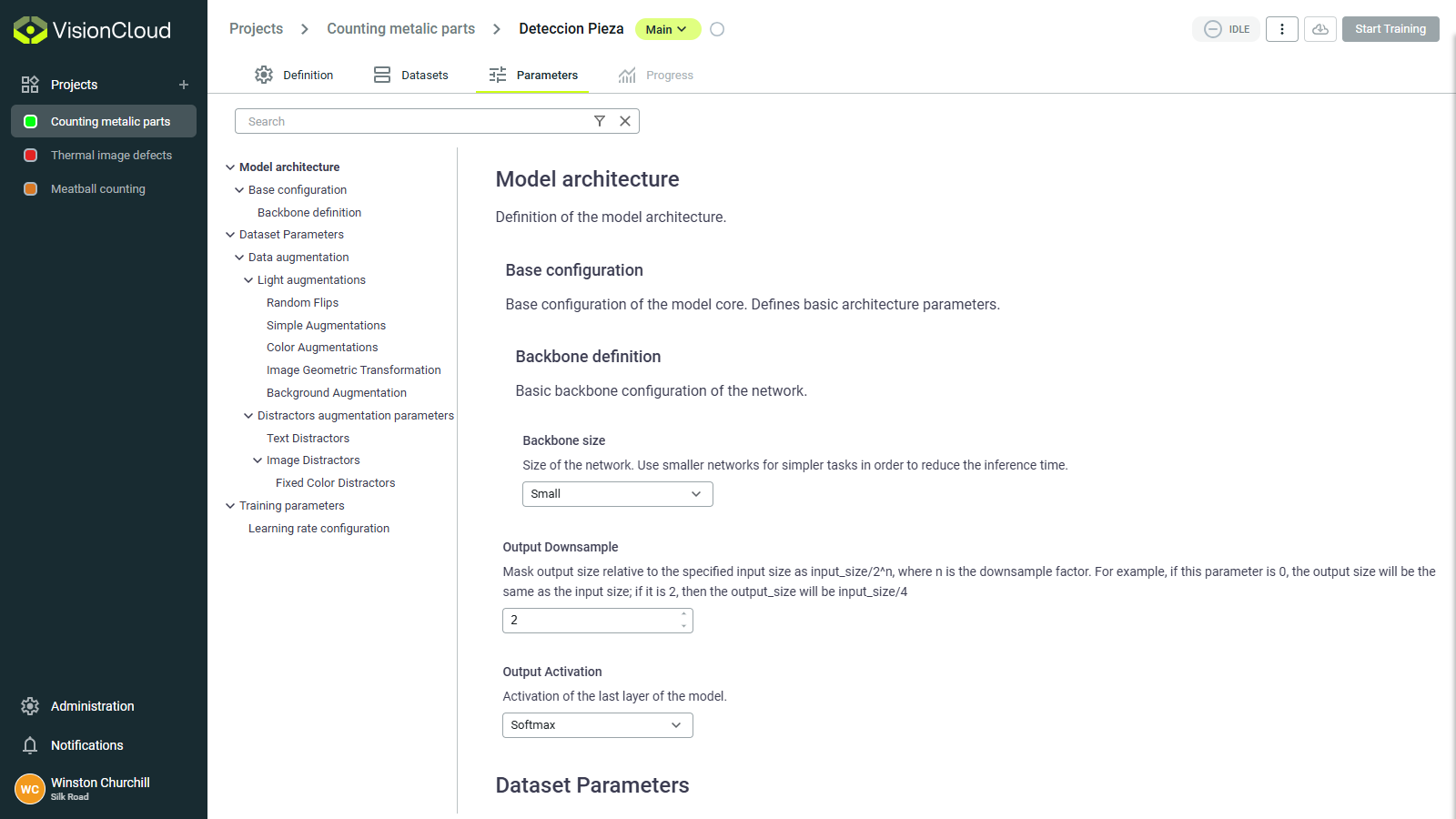
Model architecture
Define the fundamental structure of your neural network. These choices affect capacity, speed, and learning ability.
Backbone selection
The backbone is the pre-trained neural network that serves as the foundation for your model. Different backbones offer different tradeoffs between accuracy and computational efficiency:
| Backbone family | Characteristics | Best for |
|---|---|---|
| Simple | Simple and fast, but limited in capacity | Basic classification tasks |
| ResNet-Simple | Custom implementation of ResNet | Complex classification tasks |
| ResNet | Good feature extraction, residual connections prevent vanishing gradients | General purpose, excellent starting point for most tasks |
| VGG | Simple architecture, strong feature extraction | Tasks requiring fine-grained visual features |
| DenseNet | Dense connections, parameter efficient | Complex visual tasks with limited training data |
| EfficientNet | Optimized for efficiency, scales well across different sizes | Mobile applications, resource-constrained environments |
| Densenet | Dense connections, parameter efficient | Complex visual tasks with limited training data |
Decision guide:
First model? → ResNet-Simple
Limited resources? → EfficientNetB0
Complex task + lots of data? → ResNet50 or DenseNet
Need fine details? → VGG
For most industrial applications, ResNet50 provides an excellent balance of accuracy and performance. Only switch to more complex backbones if you have sufficient data and computational resources.
Backbone size
The backbone size determines the depth and complexity of the neural network. Larger backbones can learn more complex features but require more memory and computation.
| Size option | Characteristics | Best for |
|---|---|---|
| Small | Fewer layers, faster training, lower memory usage | Simple tasks, limited data |
| Medium | Balanced depth and complexity | Most general tasks |
| Large | More layers, higher capacity | Complex tasks with large datasets |
| Extra large | Deepest networks, highest capacity | Very complex tasks with abundant data |
Quick selection:
- ✅ Start with Medium for most tasks
- ⬇️ Go Small if you hit memory errors
- ⬆️ Go Large if accuracy plateaus and you have more data
How to choose:
- For simple tasks or limited resources: Start with Small or Medium
- For general tasks with moderate data: Medium or Large
- For complex tasks with lots of data: Large or Extra Large
- If you encounter out-of-memory errors during training: Decrease the backbone size
Output downsample
The output downsample factor controls the spatial resolution of the model's output feature maps. Lower downsample values retain more spatial detail but increase memory usage.
| Downsample factor | Characteristics | Best for |
|---|---|---|
| 4x | High resolution output, more detail | Segmentation tasks, small objects |
| 8x | Balanced resolution and memory usage | Most tasks, good default choice |
| 16x | Lower resolution output, less detail | Large objects, classification tasks |
How to choose:
- For segmentation or tasks requiring fine detail: Use 4x or 8x.
- For general tasks: 8x is a good starting point.
- For classification or large objects: 16x to save memory.
- If you encounter out-of-memory errors during training: Increase the downsample factor.
Loss configuration
The loss function measures how far your model's predictions are from the true values, guiding the learning process:
Classification loss options:
- Cross entropy: Standard loss for classification, works well for balanced classes.
- Focal loss: Focuses on hard examples, useful when classes are imbalanced.
- Binary cross entropy: Used for multi-label classification where multiple labels can apply.
Segmentation loss options:
- Dice loss: Measures overlap between predicted and true masks, good for imbalanced pixel classes.
- IoU loss: Based on Intersection over Union, robust to class imbalance.
- Cross entropy: Can be used for segmentation but may struggle with class imbalance.
Detection loss options:
- Combination of regression losses (for bounding box coordinates) and classification losses (for object classes).
How to choose:
- For balanced classification tasks: Cross Entropy.
- For imbalanced classes (some classes appear much more frequently): Focal Loss.
- For segmentation with varying sized objects: Dice Loss or IoU Loss.
Dataset parameters
Dataset parameters control how your images are processed before and during training, affecting what your model "sees" during the learning process.
Data augmentation
Augmentation artificially expands your training data by applying transformations to create variations of your images. This helps your model generalize better to new, unseen images.
Common augmentations include:
| Augmentation | Effect | When to use | When to avoid |
|---|---|---|---|
| Horizontal flip | Mirrors image horizontally | Most applications | When left/right orientation matters (text, asymmetric objects) |
| Vertical flip | Mirrors image vertically | Satellite imagery, microscopy | When up/down orientation matters (most real-world objects) |
| Rotation | Rotates image by random angles | Objects that can appear at any orientation | When orientation is fixed in your application |
| Translation | Moves image along X or Y axis | Objects that can appear at different positions | When object position is fixed |
| Brightness/Contrast/Sharpness | Adjusts lighting conditions | Outdoor applications or varying lighting | High-precision color-based analysis |
| Aspect ratio | Changes the aspect ratio of the image | Objects that can appear at different scales | When scale is fixed in your application |
| Crop/Pad | Applies cropping or padding | Adding variation for more robust models | Precision measurement applications |
| Shear | Applies angular distortion | Adding variation for more robust models | Precision measurement applications |
| Color Changes | Varies colors randomly | Natural scene analysis | Medical imaging, color-critical applications |
| Background Changes | Varies background colors or patterns | Helps models to focus on foreground objects | Background-foreground separation tasks |
| Distractors addition | Adds irrelevant objects or patterns | Improves model robustness to distractions | When focusing on specific objects |
Recommended configurations:
- For general classification: Enable horizontal flip, minor rotation (±15°), brightness/contrast adjustments
- For object detection: All of the above plus minor scaling/zoom variations
- For precise segmentation: Limited augmentations - horizontal flip and subtle brightness adjustments
- For outdoor scenes: More aggressive brightness/contrast and weather augmentations
Choose augmentations that reflect realistic variations your model will encounter in production. Unrealistic augmentations can harm performance.
Training parameters
These settings control how your model learns from data during the training process.
Learning rate
The most critical training parameter - controls how quickly your model adapts to errors. Do not change this value unless you understand its impact. The default value should work well for most cases.
| Rate | Benefit | Potential problem |
|---|---|---|
| High (~0.001) | If stable, training will be faster | Loss increases or jumps erratically |
| Good (~0.0001) | Steady improvement, stable training | Loss decreases slowly |
| Too low (~0.00001) | Stable training, will not oscillate | Very slow progress, training barely improves |
Start with the default. If training is unstable (loss spikes), reduce by 10x. If progress is too slow after 20 epochs, increase by 2-3x.
Batch size
Number of images processed together in each training step.
| Batch size | Memory | Speed | Stability | When to use |
|---|---|---|---|---|
| 4 | Low | Slower | Less stable | Memory-limited GPUs |
| 8-16 | Medium | Optimal | Good | Recommended default |
| 32+ | High | Faster | Very stable | Large GPUs, simple tasks |
Rule of thumb: Use the largest batch size that fits in your GPU memory.
Epochs
Complete passes through your entire training dataset.
Max epochs: Upper limit on training duration
- Too few (< 50): Model doesn't learn enough (underfitting)
- Too many (> 500): Wasted computation
- Recommended: 100-200 epochs with early stopping
Min epochs: Minimum training duration before stopping is allowed
- Prevents premature stopping
- Recommended: 30-50 epochs
Set Max epochs to a generous number (e.g., 200) and rely on early stopping to halt training at the optimal point.
Early stopping
Automatically stops training when performance plateaus, preventing overfitting and saving time.
Key settings:
- Patience: Epochs to wait without improvement (typical: 10-15)
- Metric: What to monitor (validation loss, accuracy, IoU)
- Mode: Maximize (accuracy) or minimize (loss)
Example:
Patience: 15 epochs
Metric: Validation Loss
Mode: Minimize

→ Training stops if loss doesn't improve for 15 consecutive epochs